Previous: Theory 1 to 4
Synopsis
I like to think of theories 5 - 8 as the advanced theories, as they can be more complicated then the first 4 (especially t5), though 1 to 4 and 5 to 8 are grouped together in the guide, so I will do it as well. Except T8, I think it deserves it's own category.
Anyway, more theories to work through, some harder than others. Have fun!
PLEASE READ GENERAL GUIDE PAGE BEFORE READING THIS
Disclaimer: This is a simplified version of the guide. The guide will skip over things, and is not completely optimal. Click here for a more polished, in-depth, and optimal guide.
Rundown
Estimated time:
See each individual theory
What to do if you're stuck:
If you are stuck for more then expected. Are you:
- Just starting a theory? When buying a theory, you have to move your students from phi upgrades to the theory. This means that your phi will drop, so it will take a while for the tau to catch back up. This is most noticeable after buying t1
- Using the correct milestones? Check out the milestone route for each theory
- Publishing at the right times? Most theories you should publish under 20, except T2. The optimal pub multi's are found in each theories section
- Using the correct autoprestige and autosupremacy formula? Using the incorrect autoprestige / supremacy formula can impede progress, so make sure to check. The formulae are here
- Autosupremacy needs you to do a manual supremacy to get it working. You must re do this manual supremacy every time you open the equation menu. If you could afford some upgrades if you supremacied, you probably need to do a manual supremacy.
- Supermacying in the right places? The general rule of thumb is to supremacy whenever you can afford an upgrade.
- Buying / autobuying all variables/upgrades? With an autobuyer, or the buy all button, you can disable buying certain variables/upgrades, which would definitely impede progress, On that note,
- Using the right student distribution? Use !sigma in the discord server or use the student optimiser. Read intro to grad for more info
- Graduating in the right places? The full grad route is below
- Asking for help in the discord server? Anything not mentioned here can almost always be answered by the amazing people on the discord server
Graduation route
9k -> 9.4k -> 9.8k -> 10 -> 10.4 -> 10.6k -> 11k -> 12.4k (Skip T8) -> 13.4k -> 14k
Theory Basics
Publications are equivalent to prestiges for ft, so don't be afraid to use them. For the majority of theories, the optimal pub multi is below 20, though it varies by theory the notable exception is t2, which has an optimal pub multi in the thousands
Each theory provides tau, equal to the maximum rho you have reached. Your total tau is the product of the tau from each theory. \(\tau = \tau_1 \times \tau_2...\)
Each theory has milestones which speed up progress. You can always respec milestones and shuffle them around, so you can experiment as much as you wish. Some milestones provide instant benefits, whilst others can take longer the bear fruit. Some milestones are stronger than others
You do not have to "complete" a theory to move on to the next one, nor do you have to stop a theory when you get all milestones. Play whichever theory is fastest
How to read the milestone route:
The milestone route is a list of distributions, from top to bottom. For example: 0/0/1/0, means you should buy 1 of the 3rd milestone from the top. Sometimes, buying milestones unlocks new ones, which can change what is shown. These are presented in a list.
Here is an example distribution: 0/1/0 -> 1/1/0/0 -> 0/0/3 -> 1/1/0/1 -> 1/1/3/1
This means you should start by buying the 2nd milestone, then get the first milestone, which unlocks the 4th milestone. Then, when you get 3 milestones, respec your milestones and put them in the 3rd milestone, later, you should respec those milestones out of the 3rd milestone and put them in the 1st, 2nd, and 4th milestones. Finally, the next 3 milestones should go into the 3rd milestone
Common strategies:
There are some strategies that appear in many/all theories:
Doubling strats are strats where you hold off buying stepwise variables to save up for more powerful doubling variables, by only buying stepwise variables at 10x less than doubling variables. They will usually have a d after their name. For example: t1d is the doubling strat for t1 (used only in 0-1e25), where you buy the stepwise variables \(q_1\) and \(c_1\) only when they are 10x lower than the cheapest doubling variable (\(min(q_2, c_2)\)) in order to save up for them
Competing variables is when variables are added up. This means that the lower variable is "weaker" than the higher variable, because increasing it has less of an affect. Take this example: \(\dot{ρ} = c_1 + c_2\), where \(c_1\) and \(c_2\) are both doubling variables. If \(c_1 = 10\), and \(c_2 = 1\) million, obviously, increasing \(c_1\) to something like 20, even though it's being doubled, has not much of an affect. Therefore, one should not buy \(c_1\)
Levels of activeness
- Active: Actively playing the game, performing active strats
- Idle: Can check in to publish the theory every so often (best is like 10 - 20 mins but can be longer)
- Overnight: Not checking the game for over many hours
Note that even though these levels of activeness are given, it is almost always to play a new theory a good amount (~1e100 tau) although if you don't reach that when you unlock the next theory MOVE ON
It as always best to use the theory simulator to find out what theory to push.
For info on the thoery sim read here
Other:
- I'm calculating what my ρdot should be and it's not matching up! Remember, you have to include your pub multi in this calculation
- What does \(\dot{\rho}\) mean? Explained in T2 overview, even though it's briefly in T1, \(\rho\) increases by \(\dot{\rho}\) every second
Theory 5 - Logistic Function
- Expected time: 3 - 7 days, however T5 is terrible idle so it can take WAY longer
- Local Grad Route: 9k -> 9.4k -> 9.8k -> 10k
- Stuck? Read the General Info
- Milestone route: 0/1/0 -> 3/1/0 -> 3/1/2
OneTwo sentence description: Very interesting theory. Be careful, though it's necessary to buy, c2 can take more than it give.
T5 overview:
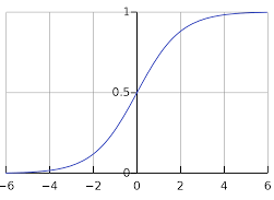
T5 is based off of a logistic function. A logistic function is a function that grows slowly at the start, speeds up, and then slows down again as it converges to some value, called it's "cap". below is the graph of a logistic function. When the value of the logistic function is far below the cap, the growth is exponential, and then as it approaches the cap is slows down exponentially, never quite reaching it
Equation Breakdown
\(\dot{\rho} = q_1q_2q\)
\(\dot{q} = (\frac{c_1}{c_2})q(1 - \frac{q}{c_2})\)
After \(c_3\) unlock
\(\dot{q} = (\frac{c_1}{c_2})q(c_3 - \frac{q}{c_2})\)
This first section is a simple equation. Increase \(q_1\), \(q_2\), and \(q\) to increase \(\rho\). The interesting part of these equations is the \(\dot{q} = (\frac{c_1}{c_2})q(c_3 - \frac{q}{c_2})\) part. This part can be split into 3 sections that are multiplied together:
- \((\frac{c_1}{c_2})\): This means that increasing c1 increases q growth and increasing c2 decreases q.
- q: This means that increasing q increases qdot. This is the "speeds up in the middle" part of a logistic function. Furthermore, this is what makes it look exponential when it is far from the cap, as having the derivative of a function be a proportional to itself is a key property of exponential functions
- \(c_3 - \frac{q}{c_2}\): This is the "cap" that q has. As q increases, this section tends towards zero, slowing down q growth, and equals zero when \(q = c_2c_3\), stopping q growth, as the 3 terms are multiplied together. Thus q can never increase past \(c_2c_3\), capping q.
From this one can understand what each variable does, and how q works:
- \(q_1\) increases rhodot when bought (~7% increase)
- \(q_2\) doubles rhodot when bought
- \(c_1\) increases q growth speed when bought
- \(c_2\) doubles q cap when bought, but halves q growth speed
- \(c_3\) doubles q cap when bought
q increases slowly, then speeds up until it reaches (about) half it's cap and then slows down as it approaches it's cap, never surpassing it.
T5 is also the second fastest theory in endgame
Bicycle analogy
Written by Playspout
Think of buying \(c_1\) as throttling on the bicycle faster. Buying \(c_2\) is similar to shifting the bicycle gear up by 1 gear. If all we do is buy \(c_1\) and never \(c_2\), then we’re stuck in gear 1 forever and make no progress. However, if all we do is buy \(c_2\) and never \(c_1\), then this is similar to trying to ride from highest gear from 0 speed, which we know takes a long time and a lot of effort. Therefore using the bicycle analogy, we should buy \(c_2\) only when we have the speed to support it; not too early and not too late. Furthermore, later in the publication, we should buy only 1 level of \(c_2\) at a time. We should buy \(c_1\) only right after buying \(c_2\) (shifting up gear).When deciding when to buy \(c_1\), \(c_2\), think of \(c_1\) as throttling a bicycle, and \(c_2\) as shifting up gear by 1 level.
Optimal publication multiplier:
t1's pub multi has no best fit, as it fluctuates a lot, but here is known:
- around 3 until 1e25
- 6 - 10 until max milestones
- Use the theory sim after that
Theory pushing
- Active: T5
- Idle: T5 EXCEPT recovery must be done active, if in recovery do T34 until 1e150 on both then T2
- Overnight: T2 until 1e400 then T4
Strategies:
Because of the drawbacks of \(c_2\), T5 benefits the most from active play. Manual \(c_2\) buying is almost mandatory when doing T5
Warning: do NOT overnight this theory. It has terrible decay past a good pub multi, and will not give good results.
All strategies revolve around increasing q as fast as possible, with doubling strats for \(q_{12}\). Before learning strats one must understand manual \(c_2\) buying during recovery
Manual \(c_2\) purchase during recovery
- Autobuy everything except \(c_2\)
- Set buy amount to x1 or x10 if over 1e150
- If q is capped (i.e. not changing) buy \(c_2\) (when \(c_2\) purchases slow down set it to x1 if it was set to x10)
- Note: You will have to spam it early in recovery just make sure not to spam it too much
- At e5 from recovery you can safely autobuy \(c_2\)
Remember to untick \(c_2\) autobuy at the end of a publication before you click publish!
Alt. Manual \(c_2\) purchase during recovery
This strategy is NOT recommended, and may cause this section to last longer than expected
You can set your buy amount to xmax instead of x1 or x10. This means that after every \(c_2\) purchase, the downside of \(c_2\) will cause q to not move for a while. For this strategy, instead of spamming \(c_2\) buy a round of it. Wait a while and buy it again. This means you could almost semi-idle it, buy not quite, as it is still pretty active (check every minute)
After manual buying \(c_2\) there are different strategies for what you do after. This strategies are seperated by activity. T5AI is active, T5 idle is (slightly confusingly) semi-idle, and T5 is idle
T5AI
| \(q_1\) | Buy at 15% of \(min(q_2 cost, c_2 cost, c_3 cost)\) |
| \(q_2\) | Always buy |
| \(c_1\) | Buy at 15% of \(min(q_2 cost, c_2 cost, c_3 cost)\) IF AND ONLY IF q is not capped |
| \(c_2\) | Always buy |
| \(c_3\) | Always buy |
T5Idle xexxx
| var | Before xexxx \(\rho\) | After xexxx \(\rho\) |
|---|---|---|
| \(q_1\) | Always buy | Always buy |
| \(q_2\) | Always buy | Always buy |
| \(c_1\) | Always buy | Never buy |
| \(c_2\) | Always buy | Always buy |
| \(c_3\) | Always buy | Always buy |
The value xexxx is found in the theory simulator. If not using the theory sim it is usually 10x higher then the last pub poin, i.e. if you published at 1e100 then stop buying \(c_1\) at 1e101
T5
Full Autobuy
Theory 6 - Integral Calculus
- Expected time: 2 - 5 days
- Local Grad Route: 10k -> 10.4k -> 10.6k -> 11k
- Stuck? Read the General Info
- Milestone route: 0/1/0 -> 1/1/0/0 -> 1/1/1/0 -> 1/0/0/3 -> 1/0/1/3 -> 1/1/1/3
- One sentence description: Looks complicated, but just a polynomial with extra steps
T6 overview:
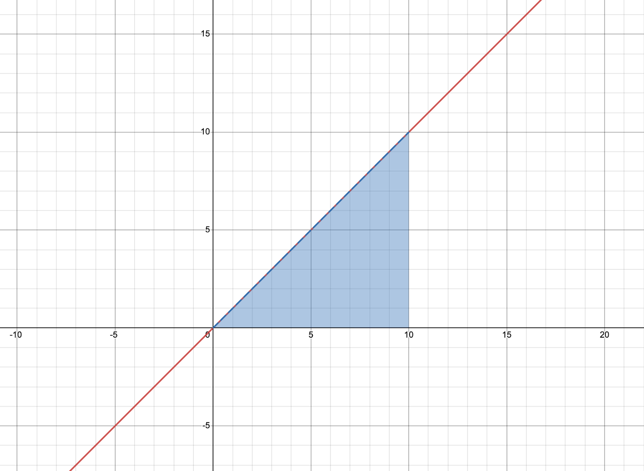
T6 is based on the idea of a definite integral. A definite integral finds the area under the graph of an equation from 2 points. Before a new dimension is bought, it's finding the area under the graph of a 2d expression (q, f(q)), after it is bought, the graph moves into 3d (q, r, f(q,r)).
For example, let's take the equation f(x) = x. The graph f(x) = x is just a line. The area under the line from 0 to 10 is shown below. The integral from 0 to 10 of f(x) is the shaded area in the diagram. That is what an integral is. This can be calculated as a triangle, but there are other methods.
Equation breakdown
Using said other methods, T6's equation can be simplified to the following (remove any terms containing not unlocked variables):
\(\rho = c_1c_2q + \frac{1}{2}c_3q^2 + \frac{1}{3}c_4q^3 - C\)
\(\dot{\rho} = c_1c_2\dot{q} + c_3q\dot{q} + c_4q^2\dot{q}\)
Or after the new dimension milestone
\(\rho = c_1c_2qr + \frac{1}{2}c_3q^2r + \frac{1}{3}c_4q^3r + \frac{1}{2}c_5qr^2 - C\)
\(\dot{\rho} = c_1c_2(q\dot{r} + r\dot{q}) + \frac{1}{2}c_3(q^2\dot{r} + 2qr\dot{q}) + \frac{1}{3}c_4(q^3\dot{r} + 3q^2r\dot{q}) + \frac{1}{2}c_5(2qr\dot{r} + r^2\dot{q})\)
The -C part can be ignored, it's just there to decrease \(\rho\) when you buy an upgrade.
Optimal publication multiplier:
6 - 12
Theory Pushing
- Active: T6
- Idle: T6
- Overnight: T2 until 1e350 T2 then T6
Strategies:
Like T4, the strategies change due to variable competition and different variable taking over
- 1 - 1e25: T6C3d*
- 1e25 - 1e100: T6C4d**
- 1e100 - 1e120: T6noC34d
- 1e120 - 1e190: T6noC345d
- 1e200+: T6noC34d
*note the before 1e7 you will have to buy \(c_{12}\) because you can't afford \(c_3\)
** note that before 1e25 you will have to buy \(c_3\) because you cannot afford \(c_4\)
There is a more difficult strategy pot 1e200 called T6AI. However to simplify, I have a strategy I call T6AInoMod (renamed) or T6C5dC12rcv using descriptive names. Because it is not in the guide The sim will not recommend this strat, and people may not know it.
For the relevant idle strategy, simply autobuy all variables that are not listed as "Never Buy"
T6C3d
| \(q_1\) | Buy at 10x less then \(min(q_2 cost, c_3 cost)\) |
| \(q_2\) | Always buy |
| \(c_1\) | Never buy |
| \(c_2\) | Never buy |
| \(c_3\) | Always buy |
T6C4d
| \(q_1\) | Buy at 10x less then \(min(q_2 cost, c_4 cost)\) |
| \(q_2\) | Always buy |
| \(c_1\) | Never buy |
| \(c_2\) | Never buy |
| \(c_3\) | Never buy |
| \(c_4\) | Always buy |
T6noC34d
| \(q_1\) | Buy at 10x less then \(min(q_2 cost, c_2 cost)\) |
| \(q_2\) | Always buy |
| \(c_1\) | Buy at 10x less then \(min(q_2 cost, c_2 cost)\) |
| \(c_2\) | Always buy |
| \(c_3\) | Never buy |
| \(c_4\) | Never buy |
| \(c_5\) | Always buy |
T6noC345d
| \(q_1\) | Buy at 10x less then \(min(q_2 cost, c_2 cost)\) |
| \(q_2\) | Always buy |
| \(c_1\) | Buy at 10x less then \(min(q_2 cost, c_2 cost)\) |
| \(c_2\) | Always buy |
| \(c_3\) | Never buy |
| \(c_4\) | Never buy |
| \(c_5\) | Never buy |
T6AInoMod / T6C5dC12rcv
| var | Recovery | Tau gain |
|---|---|---|
| \(q_1\) | Buy at 10x less then \(min(q_2 cost, c_2 cost)\) | Buy at 10x less then \(min(q_2 cost, c_2 cost)\) |
| \(q_2\) | Always buy | Always buy |
| \(c_1\) | Buy at 10x less then \(min(q_2 cost, c_2 cost)\) | Never buy |
| \(c_2\) | Always buy | Never buy |
| \(c_3\) | Never buy | Never buy |
| \(c_4\) | Never buy | Never buy |
| \(c_5\) | Never buy | Always buy |
Theory 7 - Numerical methods
- Expected time: 2 - 5 days
- Local Grad Route: This section lasts until 12k but do NOT grad at 12k
- Stuck? Read the General Info
- Milestone route: 0/1/0 -> 0/1/1 -> 0/0/2 -> 0/0/3 -> 0/1/3 -> 1/1/1/1/1 -> 1/1/1/1/3
One sentencedescription: Short answer: Move a point up a steep slope fast, Long answer: it's complicated
T7 overview:
\I have recently learnt how T7 works (thankyou megaminX and 3b1b), and it's really freaking complicated.
This part is not simple at all. You don't have to read all this, you can just skip to the strategies
The function \(g(\rho_1, \rho_2)\) is a function that maps every point in \(\rho_1, \rho_2\) space to a number. You can imagine each point in \(\rho_1, rho_2\) space, raised to that number. So for example, if g(1,1) = 2, then the point 1, 1 would be raised 2 units up in the 3rd dimension. This create a surface in the 3rd dimension, a sort of 2d terrain if you will.
the \(\nabla\) is the del operator. It is the gradient of the function. You can imagine it like this: Imagine you are standing on a point. You look around and you see the terrain around you, and the gradient of the function tell you which way is uphill. Is it in the positive x direction? negative y? Some other direction? And it tells you how steep it is. Is it a cliff? or only a gentle incline.
This information is given as a vector. You can this of a vector as an arrow which is in the same spot you are, pointing uphill, and the bigger the arrow the steeper it is.
and finally we have the equation \(\dot{\rho} = q \nabla g\). This means you look in the direction the arrow is pointing and start walking. Your speed depends on q and the size of the vector \(\nabla\) g. As you walk you constantly make adjustments to your speed and directing based on the the value of \(\nabla\) g is at you new point.
A vector can be split up into x and y components, meaning if you walk in the direction of the vector, from the start of the arrow to the end of the arrow, you will have moved the vectors x component in the x direction, and the vectors y component in the y direction. In our case, we split it into \(\rho_1\) and \(\rho_2\) components
This is an example of a maximisation algorithm. It moves you to a local maximum, a point where the graph is highest, as you will always move upwards
From now on I will only use \(\rho_1\), \(\rho_2\) coordinates, not x and y.
\(\rho\) is the point \(\rho_1\), \(\rho_2\), and we will still use "you" as the thing that moving. Just remember it's actually \(\rho\)
In this example your goal is to maximise \(\rho_1\), to be as far away from the origin in the \(\rho_1\) direction. To do this you want to increase both q and the \(\rho_1\) component of \(\nabla\) g. To do this you want to be facing the steepest incline you can facing to the \(\rho_1\) direction
So, block out the \(\rho_2\) direction. You are now on a line. What you want is that when moving forwards, you find yourself moving up a very, very steep incline, the steepest you can get. To find this incline you can use differentiation (slightly different from how T2 uses it, here the derivative of a function is it's gradient). This allows you to look at a function and a point along the function and can find the gradient at a point.
Right now, we are not moving along \(\rho_2\), so we can treat \(\rho_2\) as a constant. This means that at least in our limited view, \(g(\rho_1, \rho_2)\) is just g(\(\rho_1\)). So we take the derivative of g with respect to \(\rho_1\) and we have the \(\rho_1\) direction of our \(\nabla\) g vector!
We can do the same thing for \(\rho_2\) to find the \(\rho_2\) component.
What \(\nabla\) does mathematically
Assumed knowledge: Basic understanding of vectors and differentiation
The \(\nabla\) operator is a way of taking the derivative of a multi-variable function. The function \(\nabla\)g is a function that takes in the 2 initial arguments \(\rho_1\) and \(\rho_2\) and returns a vector. As shown before this vector is found by looking at each argument individually and treating the others as constants. Thus you have the vector \(\begin{bmatrix}dg/d\rho_1\\dg/d\rho_2\end{bmatrix}\).
Equation breakdown
So finally, here are the simplified equations:
\(g(\rho_1, \rho_2) = c_1c_2\rho_1 + c_3\rho_1^{1.5} + c_4\rho_2 + c_5\rho_2^{1.5} + c_6\rho_1^{0.5}\rho_2^{0.5} \)
\(\dot{\rho_1} = c_1c_2 + 1.5c_3\rho_1^{0.5} + c_6\rho_2^{0.5} / 2\rho_1^{0.5} \)
\(\dot{\rho_2} = c_4 + 1.5c_5\rho_2^{0.5} + c_6\rho_1^{0.5} / 2\rho_2^{0.5} \)
Optimal publication multiplier:
2 - 3
Theory pushing:
- Active: T7
- Idle: T7
- Overnight: T2 until 1e350 T2 then T6
Strategy:
Despite the complexity of T7. The strategies for T7 are just standard doubling strats. with competing variables.
for idle strats simple autobuy all variables not listed as "Never Buy". The Corresponding idle strat to T7PlaySpqcayX is T7noC12
- 1 - 1e25: T7C12d
- 1e25 - 1e75: T7C3d
- 1e75 - 1e110: T7C12d
- 1e110 - 1e175 T7PlaySpqcey100
- 1e175 - 1e250: T7PlaySpqcey10
- 1e250 - 1e300: T7PlaySpqcey50
T7C12d
| \(q_1\) | When \(\frac{1}{10}\) of \(c_2\) cost |
| \(c_1\) | When \(\frac{1}{10}\) of \(c_2\) cost |
| \(c_2\) | Always buy |
| \(c_3\) | Never buy |
| \(c_4\) | Never buy |
| \(c_5\) | Never buy |
| \(c_6\) | Never buy |
T7C3d
| \(q_1\) | When \(\frac{1}{10}\) of \(c_3\) cost |
| \(c_1\) | Never buy |
| \(c_2\) | Never buy |
| \(c_3\) | Always buy |
| \(c_4\) | Never buy |
| \(c_5\) | Never buy |
| \(c_6\) | Never buy |
T7PlaySpqceyX
| \(q_1\) | When \(\frac{1}{4}\) of \(c_6\) cost |
| \(c_1\) | When \(\frac{1}{4}\) of \(c_2\) cost |
| \(c_2\) | When \(\frac{1}{X}\) of \(c_6\) cost |
| \(c_3\) | When \(\frac{1}{10}\) of \(c_6\) cost |
| \(c_4\) | When \(\frac{1}{10}\) of \(c_6\) cost |
| \(c_5\) | When \(\frac{1}{4}\) of \(c_6\) cost |
| \(c_6\) | Always buy |
Note that a higher X not only directly affects c2 buying but also indirectly affect c1 buying through c2
If there is no X, treat it as infinity, that is to use the following chart:
T7PlaySpqcey
| \(q_1\) | When \(\frac{1}{4}\) of \(c_6\) cost |
| \(c_1\) | Never buy |
| \(c_2\) | Never buy |
| \(c_3\) | When \(\frac{1}{10}\) of \(c_6\) cost |
| \(c_4\) | When \(\frac{1}{10}\) of \(c_6\) cost |
| \(c_5\) | When \(\frac{1}{4}\) of \(c_6\) cost |
| \(c_6\) | Always buy |
Note that the corresponding idle strat to T7PlaySpqcey is called T7noC12 by the theory sim
Post T7 and T8 skip
- Expected time: 3 - 5 days
- Local Grad Route: 11k -> 12.4k (skip T8) -> 13.4k -> 14k
Why do we skip T8?
T8 is very slow before 1e60, and is thus the ONLY theory where the tau it provides it outweighed by the phi that the 5 students would provide. Don't worry, you will still buy T8, just at 14k instead of 12k.
When T8 is bought, it unlocks another student upgrade: R9, as it is the ninth from the top. When you have 14k, you will be able to afford both T8 and R9. R9 boosts theory speed, and makes them faster, meaning T8 is worth it
When you reach 12k, buy T8, swap to it, and then sell it, so you can get the achievement and the 100k stars that come with it. Also, you will be able to see R9 (but not buy it)
Optimal Theory Distribution for 14k
As you push for 14k, you should not only focus on T7. The optimal theory distribution looks like this, so try to focus on theories that are lacking:
- T1: e200
- T2: e290
- T3: e130
- T4: e155
- T5: e265
- T6: e165
- T7: e145
- T8: SKIP
For overnighting use T2 until 1e350 T2 then T6. If your T6 is very high you can start moving to T4
If your numbers are slightly different that's fine. You just need about e1350 total tau to get to 14k.
For strats, please go back to the relevant sections
Next: Theory 8 and R9